The concept of VQ-VAE at first glance is seemingly counterintuitive. The paper moves away from the very reason that the model it was based on was made for in the first place, but in spite of that VQ-VAE still provides something more novel than many of the other extensions of VAEs did. This post was mainly inspired by a difficulty in learning the reasons behind the decision making rather than anything profound or interesting within the papers, although even without a need to understand the material, the ideas explored within the progression between each model are a nice and concise way to understand the implications behind the types of latent space used.

Autoencoders:

Autoencoders are the one of the most basic models within unsupervised learning. They are ubiquitous with the term and can be found in or at the very least has inspired almost every open-ended computer vision model. They are a simple type of Encoder-Decoder model, often only containing 2-3 layers, that aims to generate an interpretable latent space in between both models. This latent space acts as a lower dimensional representation of the input, and acts as an unsupervised method of generating representations for practically any modality.

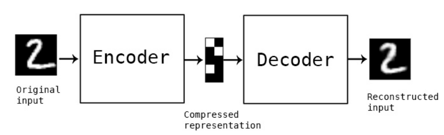
The goal of the model is to minimize a reconstruction loss between the encoder’s input and the decoder’s output. This means that the encoder aims to generate a representation of the input that is interpretable enough for the decoder to reconstruct it perfectly. Each of these representations are contained within the latent space the model provides. This structure is then extended to help fix problems with training and quality of representation generated, but the main takeaway necessary for our purposes is that these models generate an unstructured continuous space. The representations of each image, if defined as a point within this space, do not have any positional or contrastive differences. This is to say that the decoder can only ever decode images that it has been trained on, and if given an altered latent representation the model would not be able to reconstruct a similar input.

Variational Autoencoders:

This limitation of the decoder is the motivation behind Variational Autoencoders, which impose a distribution based structure on its latent space. Instead of having the encoder output an uninterpretable set of numbers, a VAE’s encoder outputs a set of distribution parameters, with each distribution having a mean $\mu$ and a standard deviation $\sigma$. The exact meanings of these in terms of the distribution do not matter much for the interpretation of the model, as they are just used as a method of keeping everything well structured.

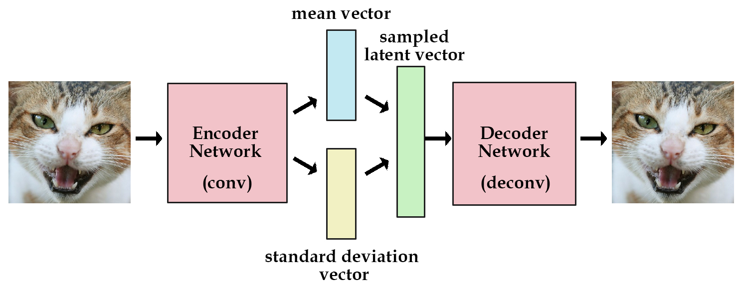
In order to keep the latent as something that has a gradient for training, the variable is reparameterized during training. This also introduces some randomness to the training in the form of a noise parameter $\epsilon$ modeled after the standard Gaussian Distribution. This both helps the model maintain the structure it desires within its latent space, but also allows the decoder to work with different perturbations of inputs outside of the ones given by the encoder.

$$z=\mu+\sigma\odot\epsilon,\space\epsilon\sim\mathcal{N}(0,I)$$

Training the model still uses the same reconstruction loss, which depends on the exact dataset used with the model, but also adds a new term to further improve the structure of its latent space. KL-Divergence is a method of determining how similar two distributions are. The term is used within VAEs to help ground the parameters of each distribution to something that is sensible, since without this term each latent representation would devolve into the same unstructured form that typical Autoencoders use. The loss pushes the distribution formed by each pair of variables towards some favorable distribution $p(x)$, often the same standard Gaussian Distribution used within the noise $\mathcal{N}(0,I)$. The combination of the reconstruction loss and the KL divergence loss creates a sort of tug-of-war that reaches a happy medium between the two, since the reconstruction loss wants complex distribution parameters that are more meaningful and the KL divergence loss wants simpler ones with less meaning.

$$\mathcal{L}_\text{VAE}=\mathcal{L}_\text{recon}+\beta\cdot D_\text{KL}(q_\phi(z|x)\|p(z))$$

All of these changes are done to create a structured continuous latent space. The main use case of VAEs is within generative AI, where the decoder’s prowess with perturbed data shines, giving it the ability to generate new data that it has never seen. This is only possible due to the structure imposed on its latent space, making slight changes within latent representations result in similar outputs.

VQ-VAE:

Although the entire purpose of these models is to generate a form of continuous space that can then be worked with and on, VQ-VAE (short for Vector Quantised Variational Autoencoder) takes these concepts and moves in the opposite direction. The model aims to generate a structured discrete space, one that is defined by a preset codebook of different values that are learned through the model’s training.

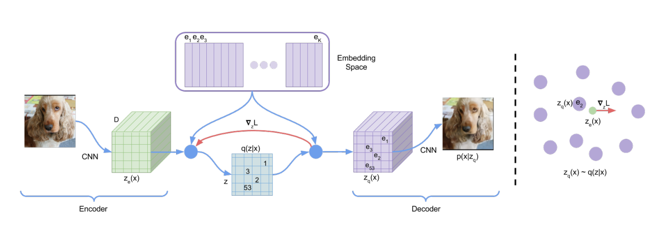
The architecture of the model stays almost the exact same as a typical autoencoder with one key difference within the intermediate steps between the encoder and decoder. The reparameterization trick and the KL divergence loss are removed from VAEs, as the borrowed name is done mainly for their shared interest in a structured latent space. The latent representations generated by the encoder are quantized, meaning they are snapped towards the nearest neighbor within this predefined codebook. This is formalized for some input $x$, an encoder $z_e(\cdot)$, and embeddings within the codebook $e$, with the final snapped latent variable being $z_q(x)$.

$$\begin{gather*} q(z=k|x)=\begin{cases}1&\text{for }k=\text{argmin}_j\|z_e(x)-e_j\|_2\\0&\text{otherwise}\end{cases}\\ z_q(x)=e_k,\text{ where }k=\text{argmin}_j\|z_e(x)-e_j\|_2 \end{gather*}$$

Training the model is used to update both the Encoder-Decoder weights as well as the codebook entries. Since the vector quantization step has no real method of generating a gradient, a straight-through estimator is used, meaning that the gradient is skipped during back-propagation. The general reconstruction loss is used to update the model, but two additional terms are added. The second term acts as a vector quantization object and aims to move dictionary terms towards the encoder outputs to update each embedding. The third term acts as a commitment loss that wants the encoder to generate outputs close to a codebook embedding.

$$\mathcal{L}=\mathcal{L}_\text{recon}+\|\text{sg}[z_e(x)]-e\|^2_2+\beta\|z_e(x)-\text{sg}[e]\|^2_2$$

This system is made to generate a learned and structured discrete latent space. This codebook acts as a discrete way to represent the dataset the model is trained on in the same way that word embeddings are used to represent the discrete patterns in language. This not only allows for models that work with discrete data to work with the model, but also allows for relationships to be formed and learned between each codebook embedding in a way that a continuous latent space does not allow for.

PixelCNN:

In order to capture how VQ-VAE is used for generation we have to very briefly cover a method of autoregressive image generation called PixelCNN, which first requires a brief overview of PixelRNN. PixelRNN is a method of converting Recurrent Neural Networks into a form of autoregressive image generation. The model turns an $n\times n$ image into a sequence $x_1,\dots,x_{n^2}$ by the image row by row. The entire image’s probability $p(x)$ is then modeled as the product of each pixel p(x_i), with each probability being that given the information from the previous pixels within the sequence.

$$p(x)=\prod^{n^2}_{i=1}p(x_i|x_1,\dots,x_{i-1})=\prod^{n^2}_{i=1}p(x_i|x_{<i})$$

Each pixel is jointly determined by three values, one for each color channel, which are also autoregressive in nature.

$$p(x_i|x_{<i})=p(x_{i,R}|x_{<i})p(x_{i,G}|x_{<i},x_{i,R})p(x_{i,B}|x_{<i},x_{i,R},x_{i,G})$$

PixelRNN achieves this type of modeling by using a system of two Long Short-Term Memory models, although the recurrent nature of these leads to issues with computational efficiency. This is where PixelCNN comes into play, which helps to parallelize the architecture by switching to a Convolutional Neural Network. The model uses a system of masks to help remain true to the autoregressive nature of the PixelRNN, which makes each pixel unable to receive information from future pixels. As well a form of gated activation is used to mimic the mechanisms within the LSTMs, with a combination of TanH and Sigmoid activations being used.

$$y=\tanh(W_f*x)\odot\sigma(W_g*x)$$

The main point of this all is to show that the model works off of discrete quantized data, most often off of pixels valued 1 to 256. With this information in mind, this model was the main one proposed for image generation using VQ-VAE. Given that the model is based on using and learning quantized data, this form of latent representation is perfect for it, used in a similar vein to how typical VAEs are used in Latent Diffusion Models, which are allowed to work on a continuous latent space due to the nature of diffusion models working in a continuous space themselves.

During training, the model considers each embedding within its codebook as equally likely to appear. The point of incorporating a PixelCNN to then act on this codebook is to develop a nonuniform prior (the probability of something to appear) over each embedding given the context of the previous, which builds a form of relationship between the embeddings within the space. This allows the PixelCNN to be given a set of codebook embeddings to generate an output that can be passed through the VQ-VAE decoder to generate an input. This helps overcome many of the model’s original shortcomings in terms of fine-grained details, as seen with the similar improvements made by Latent Diffusion models.

Conclusion:

There really is no big takeaway for this information, as again I really only wrote this because the original process of understanding each model was slightly confusing given that, even though each is quite literally named after the previous, they often only ever share a semblance of a purpose. If a conclusion does need to be reached, I do think that the interpretations of latent space laid out by each model provides a nice perspective on the different ways that these compressed spaces can be seen, and raises questions in the ways that the spaces can be seen in future models. With language model research wanting to move towards a form similar to the learned priors of VQ-VAE, one must imagine that a discrete latent space would work amazingly with the already discrete patterns of language, however one must also imagine that an even better system may exist waiting to be discovered.