Kolmogorov-Arnold Networks are one of if not the only modern example of a competitor to the Neural Network, something that has become so ubiquitous with the field of AI that it is almost entwined with the name. As the need for complexity grows higher and the computational power of our machines grows larger, KANs give an alternative that is theoretically more efficient and readable at the expense of longer training times. These networks also provide a good method of gaining insight into the purpose that a neural network serves.

Universal Approximation Theorem:

Neural Networks were derived and serve as function approximation tools. Given some unknown continuous function $f(x)$, the Universal Approximation Theorem denotes that there exists some neural network $\hat{f}$ whose difference with the original function is arbitrarily small. This is formalized for all values of $\epsilon>0$ with a non-perfect but much simpler representation of the theorem.

$$\forall x|f(x)-\hat{f}(x)|<\epsilon$$

For clarity’s sake, a neural network $\hat{f}$ is a collection connected neurons with learned linear functions (weight values $w$ in between each neuron and bias values $b$ at each neuron) with a non-linear activation function in between layers of neurons that determines which information is passed to the next set. The activation functions provide a method of non-linearity, since without them the model would only be limited in the complexity of functions it could approximate.

$$\hat{f}=\sum^N_{i=1}\alpha_i\sigma(w_i\cdot x+b_i)$$

The Universal Approximation Theorem does not guarantee or say anything about the nature or size of the Neural Network required to approximate the said function, only that one exists. Almost the entirety of AI research has been in search of methods that make the number of neurons necessary lower. One of the clearest examples is the entirety of the Transformer architecture, which adds features and layers to its structure to either stabilize or speed up training.

Kolmogorov-Arnold Representation Theorem:

The Kolmogorov-Arnold Representation Theorem is similar in concept and purpose to KANs as the Universal Approximation Theorem does to Neural Networks. Unlike the Universal Approximation Theorem, this theorem predates its model by about 60 years. The theorem states that any multivariate continuous function can be represented as a superposition of many single variable continuous functions. This is formalized for a function $f:[0,1]^n\rightarrow\mathbb{R}$ of $n$ inputs, and two classes of function $\phi_{q,p}:[0,1]\rightarrow\mathbb{R}$ (inner functions) and $\Phi_q:\mathbb{R}\rightarrow\mathbb{R}$ (outer functions).

$$f(x)=f(x_1,\dots,x_n)=\sum^{2n}_{q=0}\Phi_q\left(\sum^n_{p=1}\phi_{q,p}(x_p)\right)$$

Although within the theorem it explicitly states the number of linear functions required, within a machine learning perspective using this theorem still gives us no information about the minimum size of a model, as we don’t know the underlying function or the number of parameters it would have. For its use case in KANs, this theorem just acts as a way to guarantee that a solution to any multivariate function exists in this format.

Kolmogorov-Arnold Networks:

A KAN uses this theorem and has each neuron connection represent one of these functions and each layer representing some class of function. In classical neural network terms, the biases and activations are removed and the weights are turned into a form of non-linear function instead of a scalar multiplication. Although having removed activation functions, KANs still use much of the neural network terminology with each neuron is said to have a preactivation (its value before the weights are applied) and a postactivation (its value passed through one of the connecting functions).

Each layer $\Phi$ of the network is defined with a matrix of 1D functions $\phi$ with some form of trainable parameters, denoted for $n_\text{in}$ inputs and $n_\text{out}$ outputs (where $p=1,2,\dots,n_\text{in}$ and $q=1,2,\dots,n_\text{out}$) as $\Phi=\{\phi_{q,p}\}$. This means that the original representations theorem can be represented by two of these layers. The layer progression can be formalized with the $i$-th neuron in the $l$-th layer denoted as $(l,i)$ and its value $x_{l,i}$. This means that the preactivation of the function $x_{l,i}$ gets turned into the postactivation $\tilde{x}_{l,j,i}\tilde{x}_{l,j,i}=\phi_{l,j,i}(x_{l,i})$ where $\phi_{l,j,i}$ is the function from the $i$-th neuron in layer $l$ to the $j$-th neuron in layer $l+1$. The activation value of the next layers neurons is simply the sum of all incoming postactivations.

$$\begin{gather*} x_{l+1,j}=\sum^{n_l}_{i=1}\tilde{x}_{l,j,i}=\sum^{n_l}_{i=1}\phi_{l,j,i}(x_{l,i})\\ x_{l+1}=\begin{pmatrix}\phi_{l,i,i}(\cdot)&\phi_{l,1,2}(\cdot)&\dots&\phi_{l,1,n_l}(\cdot)\\ \phi_{l,2,1}(\cdot)&\phi_{l,2,2}(\cdot)&\dots&\phi_{l,2,n_l}(\cdot)\\ \vdots&\vdots&&\vdots\\ \phi_{l,n_{l+1},1}(\cdot)&\phi_{l,n+1,2}(\cdot)&\dots&\phi_{l,n_{l+1},n_l}(\cdot) \end{pmatrix}x_l \end{gather*}$$

Using this notation the general architecture of a KAN can be formalized. A KAN is simply a function composition of each layer $\Phi$ and its collective transformations $\phi$ on the input. This can also be reformatted as $f(x)=\text{KAN}(x)$ to better show the implication and relationship with the original theorem.

$$\begin{gather*} \text{KAN}(x)=(\Phi_{L-1}\circ\Phi_{L-2}\circ\dots\circ\Phi_1\circ\Phi_0)x\\ f(x)=\sum^{n_{L-1}}_{i_{L-1}=1}\phi_{L-1,i_L,i_{L-1}}\left(\sum^{n_{L-2}}_{i_{L-2}=1}\dots\left(\sum^{n_1}_{i_1=1}\phi_{1,i_2,i_1}\left(\sum^{n_0}_{i_0=1}\phi_{0,i_1,i_0}(x_{i_0})\right)\right)\dots\right) \end{gather*}$$

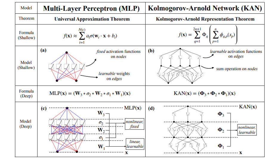
The rest of the architectural design is left up to the model’s design, but the original paper chooses each function to be B-Spline, a type of function that is controlled by a set of control points (with its behavior then being formed by the B-spline basis functions $B_i$ which are static) and a separate SiLU activation. This is defined to have trainable parameters $w_b$ and $w_s$ to control the magnitude of each function along with the spline’s coefficients (the parameters of each aforementioned control point) $c_i$.

$$\begin{gather*} \phi(x)=w_bb(x)+w_s\text{spline}(x)\\ b(x)=\text{silu}(x)=x/(1+e^{-x})\\ \text{spline}(x)=\sum_ic_iB_i(x) \end{gather*}$$

The rest of the paper goes into some theoretical analysis of the model, but as I skipped over the proofs of both theorems in this post, I will also be skipping over the explorations of the differences, but this architecture does provide two main benefits each at the cost of extra training time. The learned functions allow for more human readability and understanding of the model progression and due to having less working pieces, KANs have smaller computation graphs. The paper also goes into two training techniques that further improve the model to produce the results that they do.

1. Grid Extension (training larger splines with smaller ones)
2. Simplification (a form of pruning and function selection)

Grid Extension:

A KAN wants to have splines that are as complex as possible as to help improve their performance and behavior in between control points, with the grid of a spline referring to how its control points are set up. This is where Grid Extension is introduced, which allows coarse grid splines (those with little control points) to be trained on the data and later be used to refine fine grid splines, since the complexity of the spline is dependent on how many control points are available.

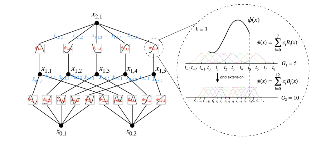
Formally, the spline wants to approximate a 1D function $f$ on a bounded region $[a,b]$ and is trained to do so with a coarse grid with $G_1$ control points separated throughout the region. In order to ensure that the behavior near the boundaries $a$ and $b$ is well-defined, an additional $k$ points are added on both ends.

$$\begin{gather*} \{t_0=a,t_1,\dots,t_{G_1}=b\}\\ \{t_{-k},\dots,t_{-1},t_0,\dots,t_{G_1},t_{G_1+1},\dots,t_{G_1+k}\} \end{gather*}$$

Using these points the B-spline for the connection can be defined with $G_1+k$ B-spline basis functions (since each is and has to be non-zero on an interval $[t_{i-k},t_{i+1}]$). This also means that a set of $G_1+k-1$ coefficients $c_i$ are defined as the functions’ trainable parameters.

$$f_\text{coarse}(x)=\sum^{G_1+k-1}_{i=0}c_iB_i(x)$$

Once the coarse grid spline is trained and matches the function $f$, it can be used to model the fine grid spline. This is done by minimizing the distance between the two representations with trainable parameters $c^\prime_j$ for the fine spline.

$$\{c^\prime_j\}=\underset{\{c^\prime_j\}}{\text{argmin}}\mathbb{E}_{x\sim p(x)}\left(\sum^{G_2+k-1}_{j=0}c^\prime_jB^\prime_j(x)-\sum^{G_1+k-1}_{i=0}c_iB_i(x)\right)$$

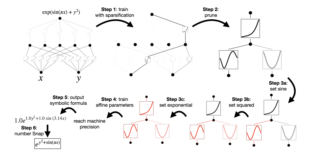
Simplification:

Due to the nature of the original theorem, if given the function that a dataset is built on, the model can be given an exactly optimal configuration. Since this is not practical and the datasets are often not interpretable to basic mathematical functions, KANs use a system of simplification to help make their models are readable as possible. The model uses a combination of three systems each used in sequence. Sparsification changes the model’s loss to favor sparsity, Pruning removes unused neurons, and Symbolification makes warps functions to form more understandable representations.

Sparsification is an extension of L1 Regularization (a regularization term that punishes large weight values) to KANs. Since the model doesn’t have scalar weights, punishing large weight values needs a different system, with the model using an L1 Norm to measure each function. The L1 Norm of a neuron $|\phi|_1$ is used to define the average magnitude of the function of $N_p$ inputs, with the L1 Norm of a layer being the sum of all of its neuron activations.

$$\begin{gather*} |\phi|_1=\frac{1}{N_p}\sum^{N_p}_{s=1}|\phi(x^{(s)})|\\ |\Phi|_1=-\sum^{n_{in}}_{i=1}\sum^{n_{out}}_{j=1}|\phi_{ij}|_1 \end{gather*}$$

As well, an Entropy term $S(\Phi)$ is defined for each layer, with the value representing the predictive uncertainty of the layer. When minimized, this encourages simpler paths through the network and wants less variance in how the information progresses.

$$S(\Phi)=-\sum^{n_{in}}_{i=1}\sum^{n_{out}}_{j=1}\frac{|\phi_{ij}|_1}{|\Phi|_1}\log(\frac{|\phi_{ij}|_1}{|\Phi|_1})$$

These are both combined with the total predictive loss $\ell_\text{pred}$ to form the loss of the model with $\mu_1$ and $\mu_2$ defining relative magnitudes along with an overall regularization magnitude $\lambda$.

$$\mathscr{l}_{total}=\mathscr{l}_{pred}+\lambda\left(\mu_1\sum^{L-1}_{l=0}|\Phi_l|_1+\mu_2\sum^{L-1}_{l=1}S(\Phi_l)\right)$$

One of the main benefits of this Sparsification penalty is that neurons that are not necessary are not involved as much within the model. In order to take advantage of this the model then uses a system of Pruning. Each neuron has an incoming $I_{l,i}$ and outgoing score $O_{l,i}$ defined (each as the maximum connection either incoming or outgoing from that neuron). If both scores are greater than a defined threshold $\theta$ (defined as $\theta=10^{-2}$ within the paper), then the neuron is deemed important, otherwise it is removed from the network.

$$\begin{gather*} I_{l,i}=\max_{k}(|\phi_{l-1,i,k}|_1)\\ O_{l,i}=\max_{j}(|\phi_{l+1,j,i}|_1) \end{gather*}$$

The last process that is done to improve readability is Symbolification. If a spline is trained and is found to resemble some known function ($\cos$, $\log$, $x^2$, etc.), the spline can be simplified to match its representation. Since the spline cannot be simply replaced with the corresponding function due to any shifts or scalings present within the spline, a set of affine parameters $(a,b,c,d)$ are trained to help fit the function $f(\cdot)$. This is done by training on a set of gathered preactivations $x$ and postactivations $y$ of the spline.

$$y\approx cf(ax+b)+d$$

Conclusion:

KANs not only present a very useful alternative to typical Neural Networks in AI architectures or another frontier of research, but they also present a very central idea that many tend to skip over. Neural Networks may and very likely are not the best method of approximating functions even as they are the golden standard as we know it today. KANs and their improvements on neural networks raise the question of whether another improvement for function approximation exists and even whether function approximation is the right choice for all of the current goals in AI. As well, the model’s ability to have a mathematically optimal model size given that a function for the dataset is given raises questions of whether assumptions can be made about the functions given more complex datasets and how that would improve these models. Overall KANs represent a method of breaking from the mold that the field is currently in, and asks those that think about the model’s potential to question whether everything they have deemed as the best option really is the best option.