When I first heard of InstantSplat and the astonishing jump in performance and efficiency that the model provides I thought someone had revolutionized Gaussian Splatting (which in case you haven’t seen, the model was shown to be able to optimize in mere seconds and be given as few as 2-3 images). I immediately put it onto my reading list and I started to theorize what the improvements could have been. After reading papers like VastGaussian and 2D Gaussian Splatting I couldn’t imagine the number of possibilities. Almost every single notable advancement made on the original Gaussian Splatting model has been made on the optimization process, but to my surprise InstantSplat didn’t do anything to the optimization process. Its ability to train several magnitudes faster and with almost no information in comparison to previous models didn’t come from any form of algorithmic or structural change, it simply just changed how and where points were instantiated, which was never brought into question by myself or in the papers I have read.

The model uses a Vision Transformer-based Siamese Network-inspired method of creating the point maps from a small subset of images. The model used, called MASt3R, extends on a previous model called DUSt3R, which will both be covered here along with the small changes made by InstantSplat.

DUSt3R:

DUSt3R (standing for Dense and Unconstrained Stereo 3D Reconstruction) is a method of multi-view stereo reconstruction (a subset of models that create a 3D model from a pair of images) that introduces the Siamese-esque Vision Transformer architecture. The model takes two images and outputs a 3D point map (with each pixel of the image being given a point within the map) along with a corresponding confidence score for each point. One of the most important benefits that the model provides is in the coordinate representation of each point map, since each point map is denoted using the same coordinate frame, specifically that of the first image.

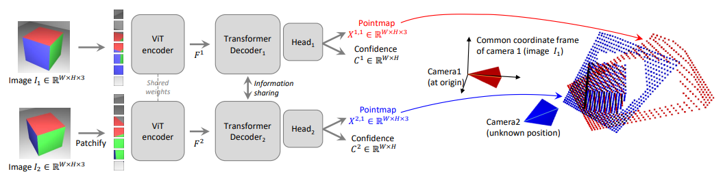
To be more specific, the model is given input images $I^1,I^2\in\mathbb{R}^{W\times H\times3}$ which yield $X^{1,1},X^{2,1}\in\mathbb{R}^{W\times H\times 3}$ (the point maps of the information from image $1$ and $2$ in the reference frame of image $1$) and confidence scores $C^{1,1},C^{2,1}\in\mathbb{W\times H}$ respectively. Each image is passed into its own Vision Transformer, although the Siamese nature described above allows each transformer to share information. First, each image is passed through the ViT Encoder of its respective model, with both encoders sharing the same weight values.

$$\begin{gather*} F^1=\text{Encoder}(I^1)\\ F^2=\text{Encoder}(I^2) \end{gather*}$$

These then get processed within a set of Decoder Blocks denoted below for some previous block outputs $G^1_{i-1}$ and $G^2_{i-1}$. As can be seen, the input to each transformer block is the state of the previous blocks from both models.

$$\begin{gather*} G^1_i=\text{DecoderBlock}^1_i(G^1_{i-1},G^2_{i-1})\\ G^2_i=\text{DecoderBlock}^2_i(G^2_{i-1},G^1_{i-1}) \end{gather*}$$

Each block also uses a system of local Self Attention (local tokens attend to other local tokens) and shared Cross Attention (local tokens attend to the other model’s tokens). For clarity this is shown below, where $\text{SelfAttention}(X^1)$ and $\text{CrossAttention}(X^2,X^1)$ can be derived by simply changing each $Q^1,K^1,V^1$ to $Q^2,K^2,V^2$ and vice versa.

$$\begin{gather*} \text{SelfAttention}(X^1)=\text{Softmax}\left(\frac{Q^1(K^1)^T}{\sqrt{d_k}}\right)V^1\\ \text{CrossAttention}(X^1,X^2)=\text{Softmax}\left(\frac{Q^1(K^2)^T}{\sqrt{d_k}}\right)V^2\\ \end{gather*}$$

Each of the outputs of the $B$ blocks is then used as input to the final decoder heads.

$$\begin{gather*} X^{1,1},C^{1,1}=\text{Head}^1(G^1_0,\dots,G^1_B)\\ X^{1,1},C^{1,1}=\text{Head}^2(G^2_0,\dots,G^2_B) \end{gather*}$$

Ground Truth Point Maps:

Before getting into how the model is trained, some clarification needs to be first provided about how ground truth point maps are derived. The model is trained on a dataset where each pair of images is given camera intrinsics $K\in\mathbb{R}^{3\times 3}$ and a depth map $D\in\mathbb{R}^{W\times H}$. These can be combined very simply to get a ground truth point map $X$ for each of the images in the dataset.

$$X_{i,j}=K^{-1}[iD_{i,j},jD_{i,j},D_{i,j}]^T$$

In order to also transform point maps into another coordinate space to match the goal made by the model, an additional set of transformations are used. World-to-Camera poses for each coordinate space $P_m,P_n\in\mathbb{R}^{3\times 4}$ and a homogeneous mapping $h:(x,y,z)\rightarrow(x,y,z,1)$ can be used to transform the point map to world space and then to the desired coordinate space. This is shown below to transform some point map $X^n$ in coordinate space $n$ to one in coordinate space $n$ $X^{m,n}$

$$X^{n,m}=P_mP_n^{-1}h(X^n)$$

Training:

The training objective for the model views the system as a method of 3D space regression. This means that the loss can be simply derived as the distance from some ground truth point and the derived point from the output. The loss repeats for valid pixels $i\in\mathcal{D}^{v}$ in view $v\in\{1,2\}$ where $\mathcal{D}^1,\mathcal{D}^2\subseteq\{1\dots W\}\times\{1\dots H\}$.

$$\ell_{\text{regr}}(v,i)=\left\|\frac{1}{z}X^{v,1}_i-\frac{1}{\bar{z}}\bar{X}^{v,1}_i\right\|$$

Both $z$ and $\bar{z}$ are normalization constants to handle the scale ambiguity of the model. Since the model does not know where the camera is the scale of the point map is hard to get very accurate. Each is derived by the average distance of the valid points to the origin.

$$\begin{gather*} z=\text{norm}(X^{1,1},X^{2,1})\\ \bar{z}=\text{norm}(\bar{X}^{1,1},\bar{X}^{2,1})\\ \text{norm}(X^1,X^2)=\frac{1}{|\mathcal{D}^1|+|\mathcal{D}^2|}\sum_{v\in\{1,2\}}\sum_{i\in\mathcal{D}^v}\|X^v_i\| \end{gather*}$$

Using this loss term however does not account for the ranging difficulty or any ill-defined points within the input, which are not assumed to be correct every time. This is counteracted by expanding the loss to be confidence-aware and uses the confidence scores from the output to scale the loss. This is shown below for a regularization hyperparameter $\alpha$ and in order to ensure that $C^{v,1}_i$ is positive, it is typically defined $C^{v,1}_i=1+\exp\tilde{C^{v,1}_i}$.

$$\mathcal{L}_\text{conf}=\sum_{v\in\{1,2\}}\sum_{i\in\mathcal{D}^v}C^{v,1}_i\ell_\text{regr}(v,i)-\alpha\log C^{v,1}_i$$

MASt3R:

MASt3R extends this architecture by including some feature mapping abilities in the model. These changes are made to make use of the improvements made by DUSt3R for tasks involving matching (merging the two point maps into one well defined one) where it was found to produce inconsistent results, which is why a much faster method of matching point maps is also derived within the paper.

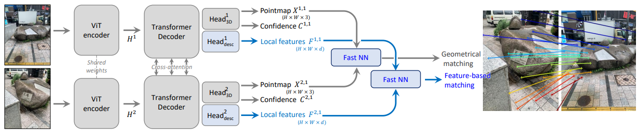
The main change in the model can be found in the prediction heads. MASt3R adds an additional pair of prediction heads to produce dense feature maps $D^1,D^2\in\mathbb{R}^{H\times W\times D}$. These are shown below and take the first block’s output and the final block’s output only instead of the entire range.

$$\begin{gather*} D^1=\text{Head}^1_\text{desc}([H^1,{H^\prime}^1])\\ D^1=\text{Head}^2_\text{desc}([H^2,{H^\prime}^2]) \end{gather*}$$

In order to encourage each feature map to have similar features, an additional loss term is added. This is defined below for a which uses a set of ground truth correspondences $\hat{\mathcal{M}}=\{(i,j)|\hat{X}^{1,1}_i=\hat{X}^{2,1}_j\}$ (points within each point map where points are shared), where $\mathcal{P}^1=\{i|(i,j)\in\hat{\mathcal{M}}\}$ and $\mathcal{P}^2=\{j|(i,j)\in\hat{\mathcal{M}}\}$ along with a temperature hyperparameter $\tau$.

$$\begin{gather*} \mathcal{L}_\text{match}=-\sum_{(i,j)\in\hat{\mathbb{M}}}\log\frac{s_\tau(i,j)}{\sum_{k\in\mathcal{P}^1}s_\tau(k,j)}+\log\frac{s_\tau(i,j)}{\sum_{k\in\mathcal{P}^2}s_\tau(i,k)}\\ s_\tau(i,j)=\exp(-\tau{D^1_i}^TD^2_j) \end{gather*}$$

This is combined with the original 3D reconstruction cost to produce the final objective for the model balanced by a hyperparameter $\beta$.

$$\mathcal{L}_\text{total}=\mathcal{L}_\text{conf}+\beta\mathcal{L}_\text{match}$$

Fast Reciprocal Matching:

The point of the feature maps is to produce a set of reliable pixel correspondences. The typical method is a system of mutual nearest neighbors, which is defined below where $\text{NN}(\cdot)$ is the function for finding a nearest neighbor.

$$\begin{gather*} \mathcal{M}=\{(i,j)|j=\text{NN}_2(D^1_i)\text{ and }i=\text{NN}_1(D^2_j)\}\\ \text{NN}_A(D^B_j)=\text{arg min}_i=\|D^A_i-D^B_j\| \end{gather*}$$

This process works very well for finding how and where both point maps match, but is extremely slow. The complexity of the algorithm is $O(W^2H^2)$ since each pixel must be compared to every pixel in the other point map. The model goes around this limitation by introducing a new iterative approach to finding these matches, which they call Fast Reciprocal Matching.

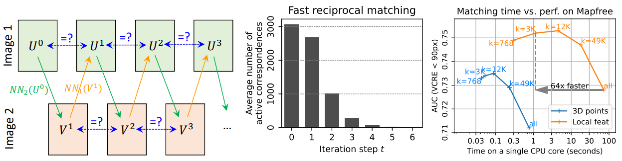
First, an initial sparse set of $k$ pixels is defined $U^0=\{U^0_n\}^k_{n=1}$ which is typically sampled on a grid in the first image. Each image is then mapped to its nearest neighbor from the second image (shown below as $V^t$). The resulting pixels are then remapped back to the first image in the same way (shown below as $U^{t+1}$). If both $U^t$ (which is $U^0$ in the first iteration) and $U^{t+1}$ are found to be the same point, they are said to have converged and are collected and removed from the process.

$$\mathcal{M}^t_k=\{(U^t_n,V^t_n)|U^t_n=U^{t+1}_n\}$$

The number of unconverged points is shown to rapidly decrease to zero after a few iterations. Once the iterations are done, the output set of correspondences is generated $\mathcal{M}_k$.

$$\mathcal{M}_k=\bigcup_t\mathcal{M}^t_k$$

InstantSplat:

InstantSplat makes a couple of key changes to the model, but they all revolve around one thing and that is the instantiation of the point cloud. If you need a refresher on the previous methods, my post about Gaussian Splatting covers it in a general sense and also goes over the optimization process so I would recommend it, but the standard method uses Structure from Motion (often shortened to SfM). SfM is a process that treats each image as a “motion” and can obtain the points of certain vertices and edges by viewing this motion. This produces point clouds that are very hard to optimize and can often have missing gaps without any points, which were often given to the optimization process to handle. I am not going to be providing any visualizations for this model and that is by choice, every single diagram I have seen has only served to confuse me and the paper does not do anything complex enough for that level of confusion to be warranted. The InstantSplat Project Site does provide some very good examples of the proficiency of the model, so I would recommend checking them out.

In order to get into the changes made by the model we first have to go over some preliminaries about the design. The model uses a system of Gaussian Bundle Adjustment which trains both the camera poses of the input images as well as the Gaussian parameters, which is necessary since the model is built to not be given any sort of positional data. When the camera poses are being trained, the rest of the model is frozen to make the process more consistent.

$$G^*,T^*=\text{arg min}_{G,T}\sum_{v\in N}\sum^{HW}_{i=1}\|\tilde{C}^i_v(G,T)-C^i_v(G,T)\|$$

Co-visible Global Geometry Initialization:

The initialization of the point cloud is handled entirely by MASt3R. No real changes are made to the model but the focal lengths across the training views are averaged to make the process more consistent.

$$\bar{f}=\frac{1}{N}\sum^N_{i=1}f^*_i$$

InstantSplat then performs some processing on this point cloud to further remove any redundancy that it can. The biggest problem point of the model is often manifested in overlapping regions, which not only increases the parameters of the representation but also slows down optimization. This is remedied by a process of View Ranking. Each view is given an average confidence score $v_i$ derived from the output confidence scores of the model and points with low enough confidence scores are pruned.

$$v_i=\frac{1}{|O_i|}\sum_{o\in O_i}o$$

These confidence scores are also used in a system they implement to derive the depth of each point. The system prunes points that have too large of a difference between some estimated projection and its original depth values. The projection is generated for some view $j$ with the point maps of views with higher average confidence scores $\{(\tilde{P}_i\in\mathbb{R}^{H\times W\times 3})\}^2_{i=1,i\neq j,v_i>v_j}$ being projected onto it. The process is shown below that generates a visibility mask $\mathcal{M}_j$ to denote the difference between the projection and original depth values, defined with a threshold hyperparameter $\theta$.

$$\begin{gather*} D_{\text{proj},j}=\bigcap_{\{i|v_i>v_j\}}\text{Proj}_j(\tilde{P}_i)\\ \mathcal{M}_j=\begin{cases}1&\text{if }|D_{\text{proj},j}-D_{\text{orig},j}|<\theta\\0&\text{otherwise}\end{cases}\\ P_j=(1-\mathcal{M}_j)\cdot\tilde{P}_j \end{gather*}$$

Optimization:

The model also uses this methodology of taking advantage of the confidence scores in the optimization process. Each point’s confidence scores are used as a gauge for how much error was in the initialized value of the point. This allows points with lower confidence scores to be changed more per step which speeds up convergence. Each confidence score first needs to be calibrated to a proper range and is scaled by a hyperparameter $\beta$.

$$O_\text{norm}=(1-\text{sigmoid}(O_\text{init}))\cdot\beta$$

The objective function is the usual photometric loss used in previous models, defined below for a 3D rasterizer $\tilde{C}(G,T)$ and ground truth $C$.

$$\begin{gather*} \mathcal{L}_\text{photo}=\|C-\tilde{C}(G,T)\|\\ (G^*,T^*)=\text{arg min}_{G,T}\mathcal{L}_\text{phot} \end{gather*}$$

Conclusion:

The performance bonuses from something as simple as changing the way that parameters are initialized raises questions for the rest of the field. Every other Gaussian Splatting paper I’ve seen didn’t question the nature of the SfM initialization as far as I remember and I can not blame them. The current state of the field of computer science research has relied on the powers of gradient descent and optimization so much that we forget to think about how these weights are initialized. Seeing the improvements that this model makes while changing something we view as trivial in other fields should make one question the methods of instantiation in natural language processing and computer vision and the potential improvements to be had by doing so.