As Large Language Models and other such autoregressive architectures become increasingly dominant over the landscape of language generation, Google has released a new model centering around a completely different paradigm, Gemini Diffusion. It presents faster generation and more coherent text over even their top models, and it starts to raise the question of whether these diffusion language models are the future of generation. I’ve already covered diffusion language models very briefly in a previous blog, but this will act as a more thorough exploration in both the foundations and the current state of the paradigm.

Autoregressive Language Modeling and LLMs:

To fully understand the impact that diffusion language models have, one must first know the basics of autoregressive generation, the paradigm used by LLMs and that which has dominated the landscape for years now. To make sure that the differences are understood, I am going to give a very very brief overview of what LLMs really do under the hood.

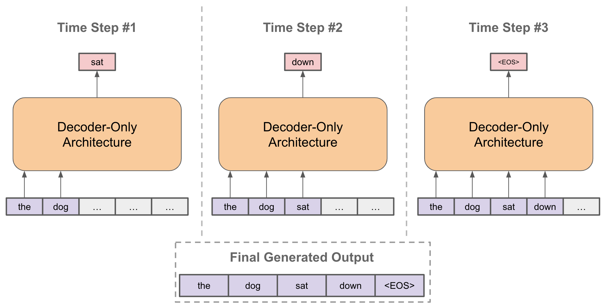
LLMs are a series of Transformer blocks, each containing an Attention block to have the information within the sequence interact and a Neural Network block to have the information be updated, which are given a sequence of tokens representing the words from the input. This is repeated however many times is deemed necessary by the model’s creators and at the very end of these blocks a final linear layer is used to get an output of probabilities. These probabilities represent the probability of a given word being next within the sequence, and the model uses these to choose the next word within said sequence. That word is appended to the input and is fed back into the model to output the next word, and for many modern LLMs this continues until a specific end-of-sentence token is output instead. This has been proven time and time again to work brilliantly, but the format is highly flawed. This style of generation is not computationally efficient in the slightest and is not backed up by how our brains are wired and process information in the slightest, being something that doesn’t use internal memory systems at all. The biggest problem that is spawned from this form of generation however is the underlying issue that the previous parts of the sequence can not be influenced by later parts.

Diffusion Models:

Diffusion Models, most often used for image and video generation, are built off of the concept of Diffusion, a concept brought from physics about structure being devolved into randomness. Instead of being trained to match an output to some given truth label, it acts to reconstruct a noisy input into its original state. This allows the model to be given an input of random noise with which it outputs a coherent image. The training of a diffusion model is broken into two parts, a forward diffusion process where noise is added to the data, and a reverse diffusion process where the model learns to remove the noise and get the original.

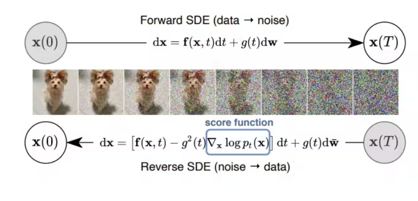
The Forward Diffusion process adds a small amount of gaussian noise to some data point $x_0\sim q(x)$ from a real dataset in $T$ steps to produce samples $x_1,\dots,x_T$. The noise is modeled after a Multivariate Gaussian Distribution and the amount of noise that is added at any given time step $t$ is defined with a Noise Schedule $\beta$ (often a hyperparameter $\{\beta_t\in(0,1)\}^T_{t=1}$).

$$\begin{gather*} q(x_{1:T}|x_0)=\prod^T_{t=1}q(x_t|x_{t-1})\\ q(x_t|x_{t-1})=\mathcal{N}(x_t;\sqrt{1-\beta_t}x_{t-1},\beta_tI) \end{gather*}$$

Reverse Diffusion then uses the model $p_\theta$ and the final noisy input $x_T\sim\mathcal{N}(0,I)$ and tries to denoise it. For small enough values of $\beta_t$, the output of $p_\theta$ can be parameterized into a Gaussian, which is shown below.

$$\begin{gather*} p_\theta(x_{0:T})=p(x_T)\prod^T_{t=1}p_\theta(x_{t-1}|x_t)\\ p_\theta(x_{t-1}|x_t)=\mathcal{N}(x_{t-1};\mu_\theta(x_t,t),\Sigma_\theta(x_t,t)) \end{gather*}$$

This leaves only two variables to be generated, the mean and variance of the distribution. The variance can be safely fixed or estimated, leaving the mean to be learned by some model $\epsilon_\theta$ (the main model of interest). This process is repeated for every pixel in the image, leaving a random amount of noise to be removed from each pixel at each timestep $t$. During inference, this process is done on an input of randomly generated noise instead of something being generated from the forward diffusion process.

$$\begin{gather*} \mu_\theta(x_t,t)=\frac{1}{\sqrt{\alpha_t}}\left(x_t-\frac{\beta_t}{\sqrt{1-\bar{\alpha}_t}\epsilon_\theta(x_t,t)}\right)\\ \Sigma_\theta(x_t,t)=\sigma_t^2I\text{ where }\sigma_t=\beta_t \end{gather*}$$

With the denoised sample being extracted, it is compared to the original. The theoretical comparison uses the KL divergence of both distributions, but this is often simplified to a straight comparison between the noise added during the forward process $\epsilon$ and the predicted noise $\epsilon_\theta(x_t,t)$.

$$\mathcal{L}=\mathbb{E}_{x_0,\epsilon,t}[\|\epsilon-\epsilon_\theta(x_t,t)\|^2]$$

The inherent randomness that comes from the random distribution sampling in the reverse diffusion process allows new images to be generated, since slight permutations in the noise from early timesteps can lead to drastically different, although still structured, outputs by the end. The exact architecture of the main model $\epsilon_\theta$ is left up to the creator’s decision, but U-Nets and Transformers are the most common choices. The exact details for image generation are not required for the rest of the blog, but the fact that the entire output is being processed together should be the main takeaway.

Classifier Guidance:

To make a model that can create images based off of a given prompt, the diffusion process has to be steered. There are a number of different ways to do this, but for our purposes in this blog the most important and simplest will be classifier guidance. A classifier model $f_\phi(y|x_t,t)$ is trained to predict labels from some noisy data. This allows the diffusion model to be given some label to generate, where the classifier model acts to define whether it is getting closer to that label or not. This is done with the gradient of the model with respect to the input at some given timestep $t$, which is used to alter the predicted noise at that given time.

$$\epsilon_\theta(x_t,t)=\epsilon_\theta(x_t,t)-\sqrt{1-\bar{\alpha}_t}\nabla_{x_t}\log f_\phi(y|x_t)$$

Classifier-Free Guidance:

This form of guidance is extended by Classifier-Free Guidance which uses a system of two models, one that denoises the input $\epsilon_\theta(z_t)$ and one that denoises the input $\epsilon_\theta(z_t,c)$ given some context $c$. At inference time, the outputs of these two models are combined using some guidance scale $w$, allowing for the importance of the given context to be dynamically controlled.

$$\tilde{\epsilon}_\theta(z_t,c)=(1+w)\epsilon_\theta(z_t,c)-w\epsilon_\theta(z_t)$$

Diffusion-LM:

At the very beginning of Diffusion Models being considered for Language Modeling, the most influential and foundational work was Diffusion-LM. The model works to provide a simple way to reformat diffusion models to the language generation paradigm with two main changes, using word embeddings and rounding.

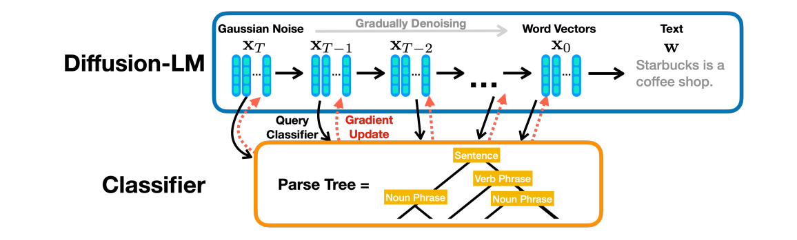
First, the text input sequence $w$ to the forward diffusion process needs to be embedded into a continuous vector space. This is done with a process of word embeddings that will feel familiar to anyone that has worked with LLMs. Each word has its own defined embedding of size $\mathbb{R}^d$. The forward and reverse diffusion processes are performed on these embeddings.

$$\text{EMB}(\textbf{w})=[\text{EMB}(w_1),\dots,\text{EMB}(w_n)]\in \mathbb{R}^{nd}$$

Once the reverse diffusion process is finished, the embedding is approximated to the nearest known word embedding. This process is shown below with an iterative argmax, although this form of rounding was not found to be sufficient within the model.

$$\text{argmax }p_\theta(w|x_0)=\prod^n_{i=1}(p_\theta(w_i|x_i))$$

With this form of rounding the word vector was often found to not commit to a single word, leading to incoherent generation. This was found as a failure of the training objective by the paper, which reformats it to incentivize the model to commit to a word as quickly as possible. Instead of being trained against the noise being added at that given timestep, the model is trained against the initial word itself. This means that the model $f_{\theta}(x_t,t)$ is constantly trying to predict the original word at each timestep, leading to a model that predicts (and therefore commits) to the word as early as possible.

$$\mathcal{L}^{\text{e2e}}_{x_0\text{-simple}}(x_0)=\sum^T_{t=1}\mathbb{E}_{x_t}\|f_{\theta}(x_t,t)-x_0\|^2$$

This form of early commitment is taken even further with something they call the Clamping Trick. At each timestep the previous timestep’s output is “snapped” to the nearest word vector. This forces the model to commit to a word during each timestep, further emphasizing the discrete nature of the text while still performing all the calculations in a continuous space.

$$\begin{gather*} x_{t-1}=\sqrt{\bar{\alpha}}\cdot\text{Clamp}(f_\theta(x_t,t))+\sqrt{1-\bar{\alpha}}\epsilon\\ \bar{\alpha}_t=\prod^t_{s=0}(1-\beta_s) \end{gather*}$$

The model is trained end-to-end (training both the word embeddings and the diffusion model) with a reformatted version of the loss function described for the diffusion models themselves. It combines the loss function from above along with a loss that moves the word embeddings closer to what the model itself predicts.

$$\mathcal{L}^{\text{e2e}}=\mathbb{E}_{q_\phi(x_0|w)}[\mathcal{L}(x_0)+\|\text{EMB}(w)-\mu_\theta(x_1,1)\|^2-\log p_\theta(w|x_0)]$$

In order to get a real language model that can function as a hypothetical generation tool, the original paper uses a simple form of classifier guidance and another network that approximates the length of the output to be generated.

LLaDA:

Standing for Large Language Diffusion with mAsking, LLaDA takes the concepts set by Diffusion-LM even further. Instead of incentivizing the model to commit to a single word in the intermediate diffusion steps, LLaDA forces the model to commit. This is done with a new paradigm of diffusion model, a Masked Diffusion Model called the Mask Predictor $p_\theta(\cdot|x_t)$.

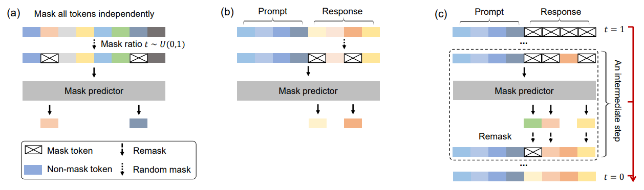
Instead of adding noise to the sequence over time, the sequence $x_0$ is masked independently, over $t\in(0,1)$ where at each timestep each token has a probability $t$ of being masked, until it is fully masked at $t=1$. The mask predictor takes any given $x_t$ and predicts all of the masked tokens $M$ simultaneously. This prediction of the mask tokens is then used in the loss function below, where $\mathbb{1}[\cdot]$ represents an indicator function which is used to show whether the token is masked or not.

$$\mathcal{L}(\theta)=-\mathbb{E}_{t,x_0,x_t}\left[\frac{1}{t}\sum^L_{i=1}\mathbb{1}[x^i_t=M]\log p_\theta(x^i_0|x_t)\right]$$

This form of diffusion does completely solve the issue with the models not committing to given words, but it brings about a different issue with the model committing too much. Any error within the generation process can not be intentionally fixed between intermediate steps, which is the problem statement made by Generalized Interpolating Discrete Diffusion for those interested, which won’t be covered here.

LLaDA then uses this paradigm with a training pattern similar to the GPT-style of LLMs, with a Pre-Training (general knowledge) and Fine-Tuning (specialized knowledge) stage. During Pre-Training, the model is given a large corpus of text data and sequences are fed randomly to it. Fine-Tuning improves the model’s use case as a language model, with it being given a pair of prompt-response data $(p_0, r_0)$. The only part that is masked during the process is the response $r_0$, and the model is trained to predict the response alone.

$$\mathcal{L}(\theta)=-\mathbb{E}_{t,p_0,r_0,r_t}\left[\frac{1}{t}\sum^{L^\prime}_{i=1}\mathbb{1}[r^i_t=M]\log p_\theta(r_0^i|p_0,r_t)\right]$$

To have a form of inference that still aligns with what the model was trained to do, LLaDA uses a system of remasking. At any given intermediate timestep from $t\in(0,1]$ to $s\in[0,t)$, after the model makes the predictions for the sequence’s tokens, $\frac{s}{t}$ of the tokens are remasked in expectation to obtain $r_s$ which is used in the next timestep. Although this should be a random process, the model uses a number of deterministic methods as well. The model also uses a system of Classifier-Free Guidance shown below with a hyperparameter $w$ for guidance scale.

$$\tilde{p}_\theta(r_0|p_0,r_t)\propto\frac{p_\theta(r_0|p_0,r_t)^{1+w}}{p_\theta(r_0|m,r_t)^w}$$

The ideas established here are extended even further by MMaDA to establish a multimodal model with a more complex training procedure, but the model won’t be covered here since the main advancements made by the model are done by copying the best practices found in LLMs (chain-of-thought, reinforcement learning, etc.), so it would require a little more explanation than what is the focus for this blog.

Conclusion:

The lengths to which this concept of Diffusion Language modeling are untold and the theoretical improvements that the paradigm provides could present something that is even more dominant in the space than LLMs. Other styles of diffusion like Diffusion Forcing and Block Diffusion that combine the strengths of diffusion and autoregression are finding more potential, but I think the main strengths of the concept come in the differences it has with autoregression. Gemini Diffusion has proven that diffusion language models generate quicker than the standards set by LLMs, but the main improvement that I have in mind is the difference in how they process information. LLMs process an entire sequence, erase their memory of the sequence, and then process the entire sequence again. This makes the generation process inherently fractured, whereas diffusion language models allow the processing to happen in the same step that the entire generation of the sequence occurs, allowing fewer memory states to affect what is being output. It gets closer to an ideal interpretable model for natural language processing and the amount of innovation that can be had with such a new technology is unknown.